22" f/4.0 lowrider
making the 6" flat secondary mirror
| home | introduction | telescope | primary mirror | secondary mirror | eq platform |
|
22" f/4.0 lowrider
making the 6" flat secondary mirror |
|
Flat
mirrors (and in the following any mirror with a radius of curvature
in the range of several kilometers or on its way to it will be a "flat" mirror
![]() )
have to meet two conditions: They should have a (spherical) surface free of
zonal defects and the radius of curvature of the sphere should be as large as
possible, in the range of several kilometers up to over 100 kilometers,
depending on size of the flat, tilting angle, and requested accuracy.
)
have to meet two conditions: They should have a (spherical) surface free of
zonal defects and the radius of curvature of the sphere should be as large as
possible, in the range of several kilometers up to over 100 kilometers,
depending on size of the flat, tilting angle, and requested accuracy.
|
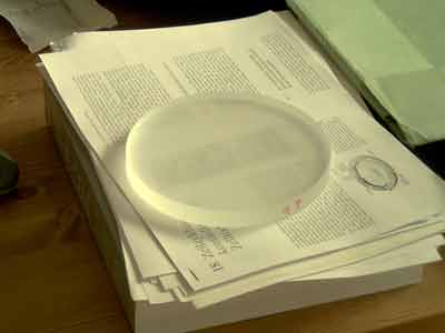
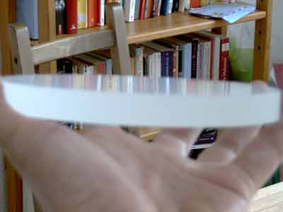
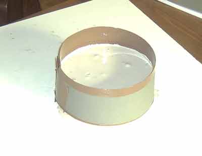
Fine grinding A flatness in the range of 1 µm can be reached by grinding three glass blanks alternatingly against each other, blank 1 on 2, 2 on 3, 3 on 1, and so on. This will be continued with each Carbo grade. After fine grinding, one of the blanks is picked as the future flat mirror and will be polished. My blanks were 150 mm borofloat blanks with 15 mm thickness from Schott, Germany. The back of the blanks should be roughened as well to prevent reflections during optical testing later on. After Carbo 1200 (right) the mirror is already reflecting under grazing angle. |
|
|
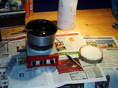
Polishing and Figuring The pitch tools were made of regular plaster. The tools were cast and sealed after complete drying for several days with several layers of clear varnish. |
|
|
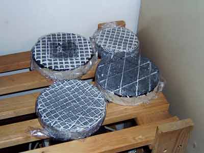
Even making pitch tools becomes routine after some time. |
|
| A finished pitch tool. The grooves were pressed into the soft pitch (heated head over in a hot water bath) using an aluminum bar. |
|
|
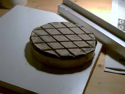
For figuring, I used at some instances special zonal polishers. In order to save my regular tool, I had prepared three tools and also had a 4 inch tool left from a previous mirror. It is quite important that your main tool has a very good fit to the extreme edge. |
|
Testing
As soon as the surface of the flat starts shining, you can start testing. I have used two different tests:
The Ritchey-Common test (RCT), which is in principle an artificial star test in the double pass against a reference sphere of long focal length. Any curvature of the flat mirror (its power, the larger the radius of curvature, the lower its power) will become obvious as astigmatism in the test setup. This is described in detail in Texerau: How to make a telescope or in the ATM book by MacKintosh: Advanced telescope making techniques (thanks to Kurt and Achim, for sending me copies!). More information on the test setup can be found further below or from Kurt Schreckling on Astrotreff.de.
The Foucault test against a reference sphere, which detects zonal errors on the surface. This is again a null test in double pass and therefore extremely sensitive.
|
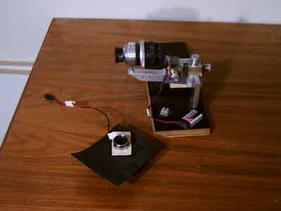
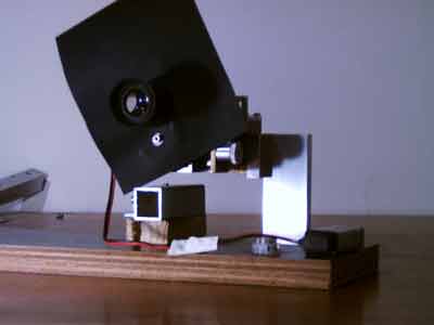
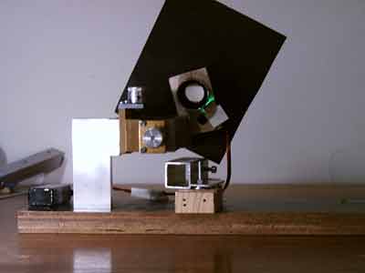
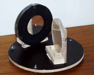
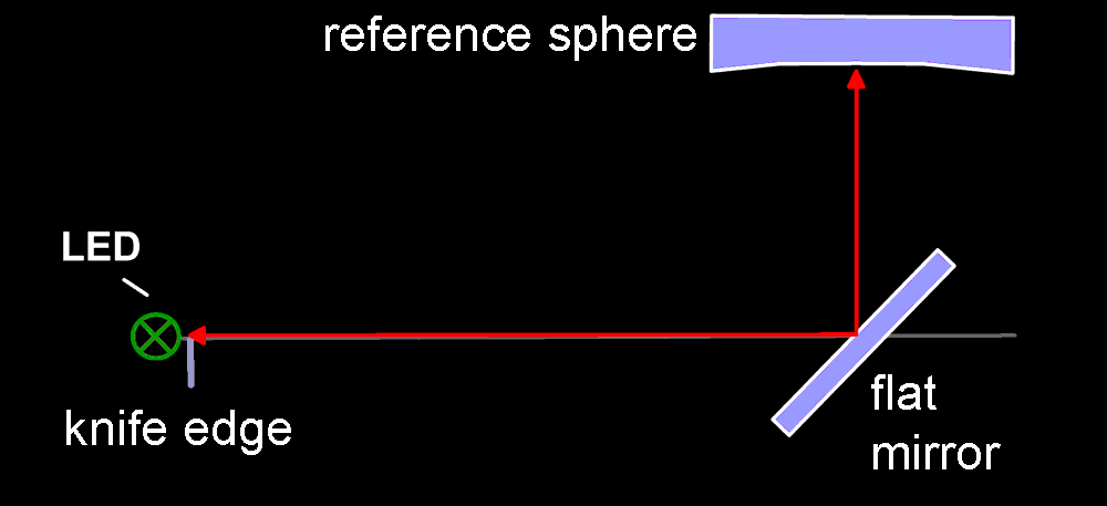
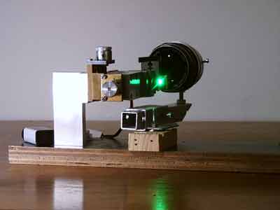
I used one and the same tester for both tests. For the RCT, I used a small pinhole in front of a bright LED and evaluated its image with a high power eyepiece. For the Foucault test, pinhole and eyepiece are replaced by a slitless Foucault setup (razor blade and LED). This switching from one test to the other should be as simple and fast as possible, since after every figuring session, the flat should be tested for both zonal errors and power. The upper picture shows the tester in slitless Foucault mode with a small accessory telescope, and with the setup for RCT lying on the table next to it. In the lower picture, the tester is shown in RCT mode with eyepiece, LED, pinhole, and a black cardboard baffle, once from the eyepiece end and once from the pinhole end. The tester can be switched between both modes using a single screw. |
|
Setup for Foucault test (slitless) against a reference sphere
| The tester in slitless mode for Foucault testing with accessory telescope. |
|
|
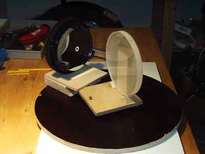
The 15 cm flat mirror with zonal mask in an approximately 90° angle to an 11cm f/4.4 reference sphere (which is a spherical as it can be). |
|
Setup for Ritchey-Common test (RCT)
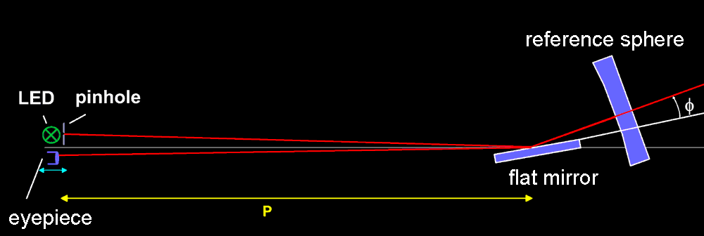
A flat mirror with non-vanishing power (i.e. with a finite radius of curvature) will give an astigmatic image of the pinhole with two focal planes, a tangential focal plane (with the rays forming a vertical focal line) and a sagittal focal plane (with the rays forming a horizontal focal line). In the Richey-Common test, the distance between both focal planes is measured.
About the pinhole: The pinhole that I used has a diameter of 10 micron. Such pinholes can be made out of aluminum foil on a piece of glass using a fine needle. Make about 20 holes and pick the best one under a microscope. Often the holes are not round, but rather cracks in the foil, which are not usable. You may encounter problems in determining the focal plains if
|
|
the pinhole is too large |
|
|
the surface of the flat deviates still strongly from a sphere (easily recognizable in the Foucault test) |
|
|
the "reference sphere" is not spherical enough |
|
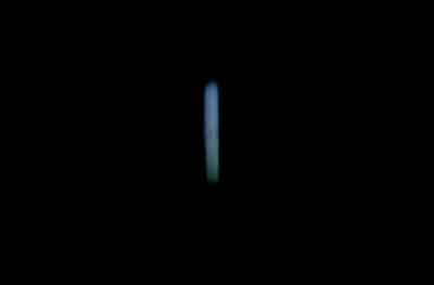
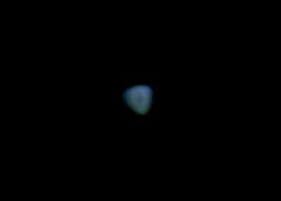
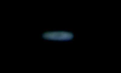
Pictures of the pinhole in the RCT
Horizontal inside / vertical outside means a convex mirror surface (Dani Steiner suggests to keep in mind: H(orizontal) I(nside) V(ertical) O(utside) CONVEX, this sounds a bit funny, is, however, easy to memorize, and that's the important point, when you are sitting behind your tester and try to remember how again to distinguish convex from concave ...) By measuring the distance x between both astigmatic foci (sagittal and tangential) you can calculate the radius of curvature of the "flat" mirror using some expressions from Texerau or Mackintosh (see below). The larger the flat mirror and the larger the angle gamma (see expression below), the stricter are the margins for the radius of curvature of the flat. As the secondary mirror of a Lowrider will be tilted by gamma~30°, corresponding to phi ~ 60°, as compared with the classical Newton (gamma = 45°, corresponding to phi = 45°), the requirements regarding the radius of curvature are not as stringent. |
outer focal plane:
between both focal planes:
close to
the inner focal plane:
|
The flat mirror of my Lowrider finally had a radius of curvature of well above 15 km, which is by far enough to avoid any visible astigmatism in the telescope. This had been confirmed as well with the optical ray tracing program Oslo LT.
In the Foucault test, the mirror had been spherical to the extreme edge with only very minor visible zonal defects (and this a null test in double pass!). However, it took me some time to get it there ...
As the ratio between small and large axis of the secondary is cos g , this yields for tilt angle g =30° a ratio of 0.87. As this is quite close to 1, I left the secondary round, yielding a smaller axis of 130 mm and a larger axis of 150 mm. The effect due to increased central obstruction is negligible.
The radius of curvature r of the flat can be calculated using the expression (see Texerau or Macintosh)
![]()
where p is the distance between the flat and the focal planes, x is the distance between sagittal and tangential focus, and phi is the tilt of the flat to the main axis (see setup in the picture further up). The sensitivity of the setup will be increased the larger p and the smaller the angle phi. (Note: The above equation is according to Texereau. My understanding is that it is for a setup with fixed light source, while the figure in the book shows a mobile light source. If you use a mobile light source, you should multiply the value of r with a factor of 0.5 (just to be on the safe side))
Using this setup, you measure exactly the optical aberration that you want to be minimized in the telescope, namely the astigmatism produced by residual power of the secondary. In my case, the tester setup was optimized for high sensitivity, such that the difference between the astigmatic foci was roughly three order of magnitudes (1000x) larger than later at work, in the telescope:
testing is in double pass, yields a factor of two
distance p was 2250 mm during testing and roughly 450 mm later in the telescope, yields a factor of 25
phi was considerably smaller during testing than later in the Lowrider, 10° compared with 60°, yields a factor of 20
| In the beginning, I performed the RCT with the same 11cm / f 500 mm reference sphere that I used in the Foucault test. The sensitivity increases, however, with the square of the distance p between flat and focus, and thus roughly with the square of the focal length of the reference sphere. In particular in the final part of figuring, a reference sphere with focal length of 500 mm was somewhat too short. |
|
|
For fine tuning, I used therefore a 20 cm / f 1200 mm parabolic mirror. The mirror was stopped down to 10 cm and later even to 5 cm, such that with a focal ration of f/12 and later f/24 it was sufficiently "spherical". The testing was performed under an angle phi of 20° and later 10°. Flat and reference sphere were fixed on an adjustable board, such that a fast switching between Foucault and RCT was warranted without the need of cumbersome alignment prior to each testing session. |
|
|
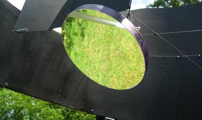
The finished secondary mirror "at work". The flat weighs roughly 800 g. Making the secondary mirror took me quite some time, but it also was very rewarding. You will learn a lot about optical theory and practical figuring techniques. I learnt, for instance, that it is quite difficult to flatten an initially slightly convex mirror without loosing the sphere. It is much easier to start with a slightly concave mirror. Luckily, you have always three blanks to choose from. I generally observed that with mirror on top (MOT), the mirror lost its sphere and its conical constant shifted below zero, even when applying only very short strokes (in other words: MOT is parabolizing). Your are therefore lacking one method to efficiently lower the center of the mirror without loosing the overall correction. By using TOT and short strokes, on the other hand, I could lower the edge slowly but smoothly and thereby flatten an initially slightly concave blank. |
|
... more flat mirrors ...
Kurt Schreckling (300 mm coelostat))
Daniel Steiner (320 mm as a testing mirror)
Richard Labschütz (170 mm)
![]()
| home | introduction | telescope | primary mirror | secondary mirror | eq platform |